

Next: Data and Evaluation
Up: Overview of the Algorithm
Previous: The Phrase Break Model
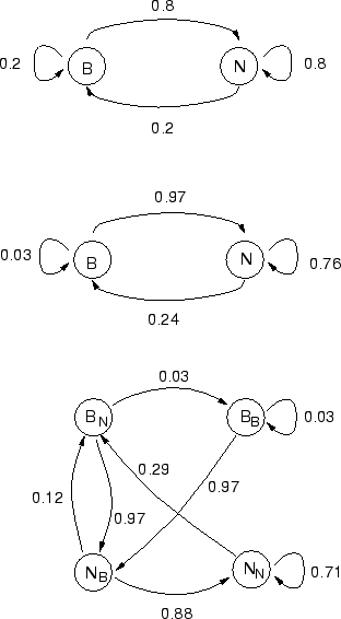
A network of TN-1 nodes and TN arcs is constructed (N=1 is
a special case and has the same topology as N=2 - see figure
1) . Each node represents a juncture type, and when
N>2 the nodes represent a juncture in the context of previous
junctures. The POS sequence probabilities do not take account of
context, and so for a given juncture type are the same no matter where
the node occurs in the network. For example, if N=3, we will have
2 break nodes, one for when the previous juncture was a break and
one for when the previous juncture was a non-break. These nodes have
the same observation probabilities. Figure 1 shows
networks for N=1, N=2 and N=3.
Figure 1:
Models for N=1, N=2 and N=3, showing actual transition
probabilities calculated from the training data. The states marked B
are for breaks and those marked N are for non-breaks. Subscripts in
state names indicate the juncture type of the previous state. In the
N=1 case the transition probabilities are just the context independent
probabilities of the juncture types occurring, i.e the transition
probabilities to a state don't depend on the previous state. In the
N=2 case, the transition probabilities take into account the previous
juncture. Thus in this model it is very unlikely that a break will
follow a break (0.03), while in the N=1 case this would still have a
relatively high probability (0.2). Looking at the probabilities of
sequences of non-breaks, we see differences in the probability of a
non-break following two previous non-breaks. As N increases, we see
that the probability of long sequences of non-breaks decreases
(
P(Ni |Pi-1, Pi-2) = 0.8 for N=1, 0.76 for N=2 and 0.71 as
N=3). Thus a higher order ngram helps prevent unrealistically long
sequences of just non-breaks or just breaks. The POS sequence model
probabilities (not shown here) are associated with each state. All
states of the same basic type are the same and so the probability
distributions for state BB (a break following a break) are the
same as for state BN (a break following a non-break).
 |
Under this formulation we have the likelihood
P(Ci|ji) (the
POS sequence model) representing the relationship between tags and
juncture types, and
P(ji | ji-1, ..., ji-N+1) (the n-gram
phrase break model) which represents the a priori probability of a
sequence of juncture types occurring. This is used to give a basic
regularity to the phrase break placement, enforcing the notion that
phrase breaks are not simply a consequence of local word information.
The probability we are interested in is P(ji) given the previous
sequence of junctures and the POS sequence at that point. This
probability can be rewritten as follows:
|
P(ji|Ci, JNi-1) = P((ji| JNi-1)| Ci)
|
(4) |
and using Bayes equation
 |
(5) |
We make the assumption that the probabilities of all states of a
particular juncture type are equal (e.g.
P(Ci | break, non-break)
= P(Ci | break, break)), so
|
P(Ci | (ji | JNi-1)) = P(Ci | ji)
|
(6) |
and from equation 5, the probability of a
juncture type given the preceding types and POS sequence becomes
 |
(7) |


Next: Data and Evaluation
Up: Overview of the Algorithm
Previous: The Phrase Break Model
Alan W Black
1999-03-20

